3.1 Finding and accessing spatial evidence
From open, cloud-based infrastructure to the GGW STAC catalog
Effective restoration decisions for large-scale, multi-country efforts like the GGW, depend on evidence that is comparable, consistent, transparent, and scalable across very different landscapes and institutions - we explored this in Module 1.1 and 1.2.
Module 2 stepped through what is meant by spatial evidence, how it is typically generated and things to consider to use it responsibly.
Now it’s time to get our hands dirty and make our own spatial evidence!
3.1.1 Data discovery and access
The shift towards open, cloud-based data
Historically, spatial datasets were difficult to discover and access - data would often sit on servers within government agencies, research institutions or commercial providers, with limited information about what data is available or how to obtain it. Obtaining it usually meant requesting a dataset and downloading it in full and working with desktop-based GIS software, which could be slow and cumbersome, particularly for large datasets.
That workflow still exists and is sometimes the most appropriate, depending on the task at hand. However it is no longer the only or often the most efficient way to work.
Earth observation and other spatial datasets are increasingly being published as open, cloud-hosted data. Instead of downloading a complete dataset before being able to use it, it can be discovered through a catalogue, queried for the parts needed, and accessed directly from the cloud.
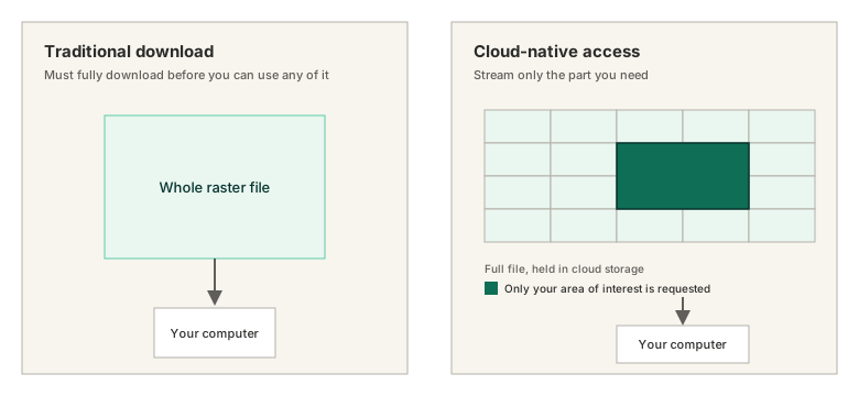
For a small dataset or one-off analysis, downloading a file may still be the most straightforward option. When working with large Earth observation archives, for example, analysing vegetation change across all 11 Great Green Wall countries over several decades, being able to discover and access data selectively can save substantial storage, download time and processing effort.
3.1.2 Sources, providers, and data formats
Open spatial data is made available in a few different ways:
- Data geoportals - government or institutional websites where we can browse and download datasets, often built around a specific country, theme, or project.
- Data catalogues - structured, searchable indexes of datasets, sometimes spanning many providers at once.
- Cloud platforms and APIs - services such as Google Earth Engine, AWS Open Data, or Microsoft Planetary Computer, which host huge volumes of data and let us query and stream it programmatically rather than downloading files individually.
Check out Ch5 - Geospatial data acquisition in Geospatial Data Science with R and Python for a more detailed overview of the different ways to access spatial data.
For further idea of the different providers and access points exist, check out this community-compiled and maintained list of open geospatial data catalogs.
Data is also stored in a range of formats and increasingly in cloud-native equivalents that make streaming and partial access possible:
| Data type | Traditional format(s) | Cloud-native equivalent |
|---|---|---|
| Raster (see 2.1.1) | GeoTIFF, PNG, NetCDF, HDF5 | Cloud Optimized GeoTIFF (COG), Zarr |
| Vector (see 2.1.1) | Shapefile, GeoJSON, KML, GPKG | GeoParquet, FlatGeobuf, Vector Tiles |
| Multidimensional / time-series | NetCDF, HDF5, GRIB | Zarr |
| Point clouds | LAS, LAZ | COPC (Cloud Optimized Point Cloud) |
The table here provides an overview of the different file format names/extension types that we’ll come across when working with open cloud-based datasets. The data in this hub is published as Cloud Optimized GeoTIFFs (COGs), which we’ll come back to shortly.
3.1.3 STAC: SpatioTemporal Asset Catalog
Alongside all these portals, catalogues, and APIs, one specification in particular has become the common language many providers now use to make their data discoverable: STAC, the SpatioTemporal Asset Catalog.
STAC began in 2017, when the Radiant Earth Foundation convened a group of around a dozen organisations including Amazon, Google, and Planet, among others working in satellite imagery and open-source geospatial software around a shared problem - every provider’s search API and data cataloguing worked differently, making it challenging to search across more than one at a time. STAC solved this with a simple, open specification for describing spatial data consistently, regardless of who publishes it. It has since been adopted by many of the largest providers of open spatial data, including major cloud and satellite platforms.
A STAC catalog organises data into a simple, consistent hierarchy:
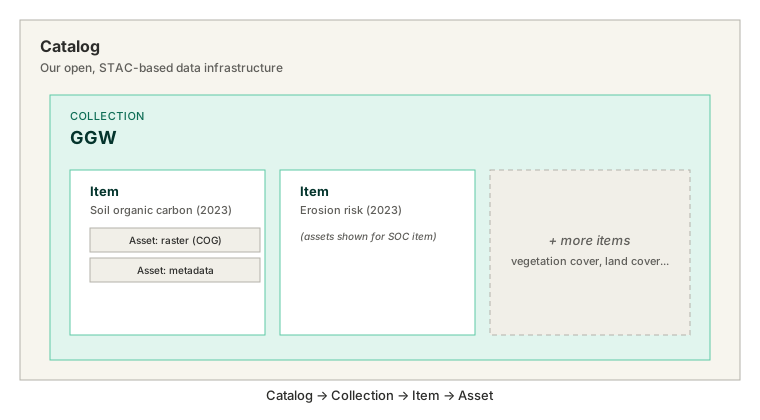
- A catalog is the top-level container - the whole data infrastructure you’re browsing.
- A collection groups together related data - for example, our GGW collection.
- An item is a single dataset within a collection - for example, the 2023 soil organic carbon prediction layer, or the erosion layer.
- An asset is an actual file attached to an item - for example, the raster itself, or its metadata.
Every item has consistent metadata describing what it represents including spatial and temporal coverage. Because this structure is the same everywhere, the same tools and approach let us discover and access data from any STAC-compliant provider instead of toying with each provider’s system, ultimately letting us answer those due-diligence questions from 2.2.2 quickly, wherever the data comes from.
Assets from STAC catalogues can be pulled into apps and web maps for visual browsing (for example, our own GGW Dashboards) which is excellent for quick exploration without writing code, but they’re best used programmatically - querying a catalogue directly from code lets us search, filter, and pull exactly the data we need into our workspace, which is the approach the rest of this module builds toward.
In this hub, we’ll refer to and use the GGW STAC collection as our main source of spatial evidence. It contains many different datasets on climate, soils, and land health, including the LDSF-based predictive models we learnt about in 2.1.
3.1.4 A worked example: accessing a GGW dataset through STAC
Here’s what discovering and accessing a dataset through our STAC catalogue looks like, step by step:
| 1. Connect to the catalog | Point your tool of choice (R, Python, QGIS plug-ins) at our STAC API endpoint, the single starting point for everything in the GGW collection. |
| 2. Search the collection | Query for the item you need, for example soil organic carbon, optionally filtered by area of interest and date. |
| 3. Inspect the result | Each match returns as a STAC item, with metadata describing what it is, coverage, and links to its assets. |
| 4. Retrieve the asset | Follow the link to the actual file, a Cloud Optimized GeoTIFF (COG) in our case, which can be streamed directly rather than downloaded in full. |
| 5. Load data | Using the COG format, you can request only the area you’re interested in, even from a file covering the whole GGW. |
This kind of workflow can be implemented using many different tools which we’ll explore in 3.2. This hub uses an R and RStudio set-up - let’s head to the next section to get started.