Notebook 2: Land Health, Soil Health and Spatial Workflows

This second notebook builds on the foundations introduced in Notebook 1 and applies them to land health, soil health, and spatial analysis data.

It shows how to move from simple tables containing coordinates to spatial objects in R, and then to static maps, interactive maps, and introductory spatial analyses that are useful for restoration planning.

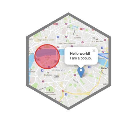
Notebook 2 is designed as a practical progression from tabular data to spatial data. Participants learn how to load and inspect datasets derived from LDSF predictive maps, convert them into spatial objects, and then produce simple maps and outputs for exploring restoration indicators.

What you will learn and do

This notebook is organised around three connected sections:

1. Loading and exploring LDSF data

The first section introduces the datasets used in the notebook and shows how to prepare them for analysis.

Load land health and soil health tables
Examine data structure, variables, and missing values
Filter data by country or area of interest
Understand indicators such as erosion, tree cover, soil organic carbon, and pH

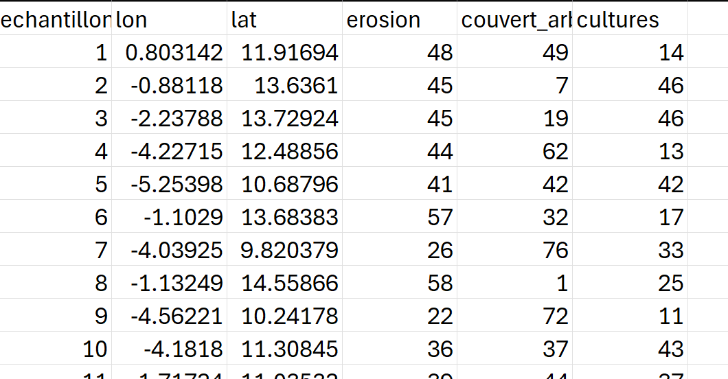
2. Moving from tables to spatial data

The second section shows how to transform data containing longitude and latitude into spatial objects that can be used in R.

Convert a table into a spatial object using sf
Understand coordinate reference systems and CRSs
Check the spatial extent of the data
Perform simple spatial operations, such as filtering points within a polygon

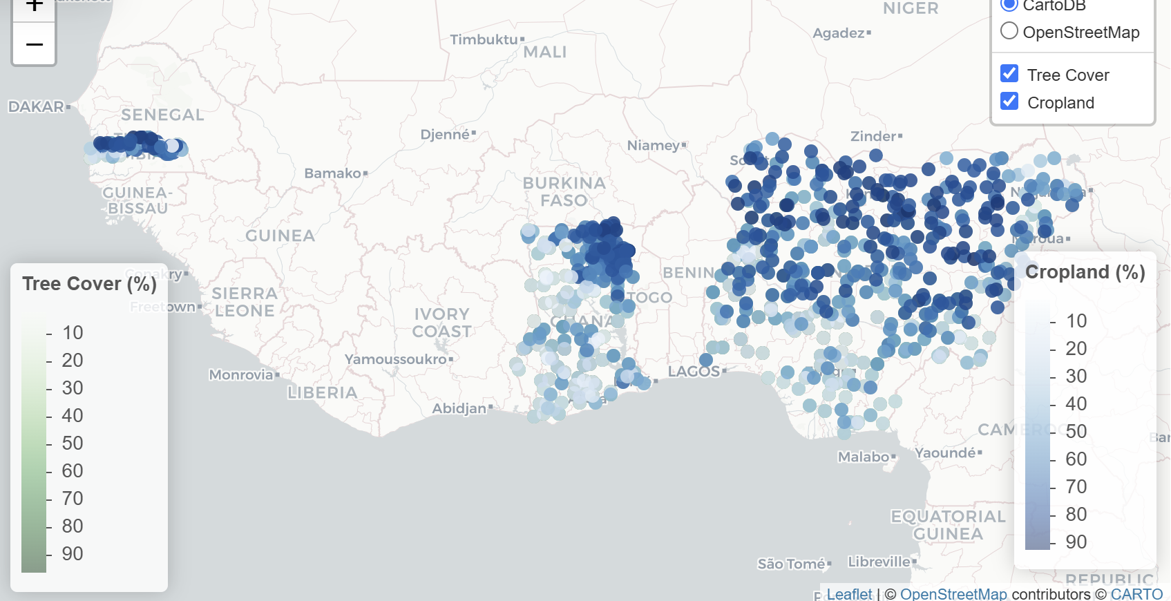
Converting tabular data into spatial data

3. Mapping and interpreting indicators

The final section uses static and interactive maps to explore spatial patterns and communicate results.

Create static maps with ggplot2 and sf
Create interactive maps with leaflet
Add colours, legends, popups, and layer controls
Export results as figures, CSV files, or GeoPackages

Interactive mapping of restoration indicators

Land health and soil health data

Land health and soil health indicators are essential for understanding the conditions that influence restoration. They help us examine landscape condition, ecological constraints, and opportunities for intervention.

In this notebook, you will work with two main datasets:

Land degradation and land cover: estimates of erosion, tree cover, and cropland
Soil health: soil organic carbon, total nitrogen, pH, sand fraction, and silt fraction

These indicators allow us to explore several important questions for restoration:

Where do erosion risks appear to be higher?
Where do we observe greater tree cover?
How do soil indicators vary between sites?
How can we combine tabular and spatial data to better understand landscapes?
How can we produce simple maps to communicate results?

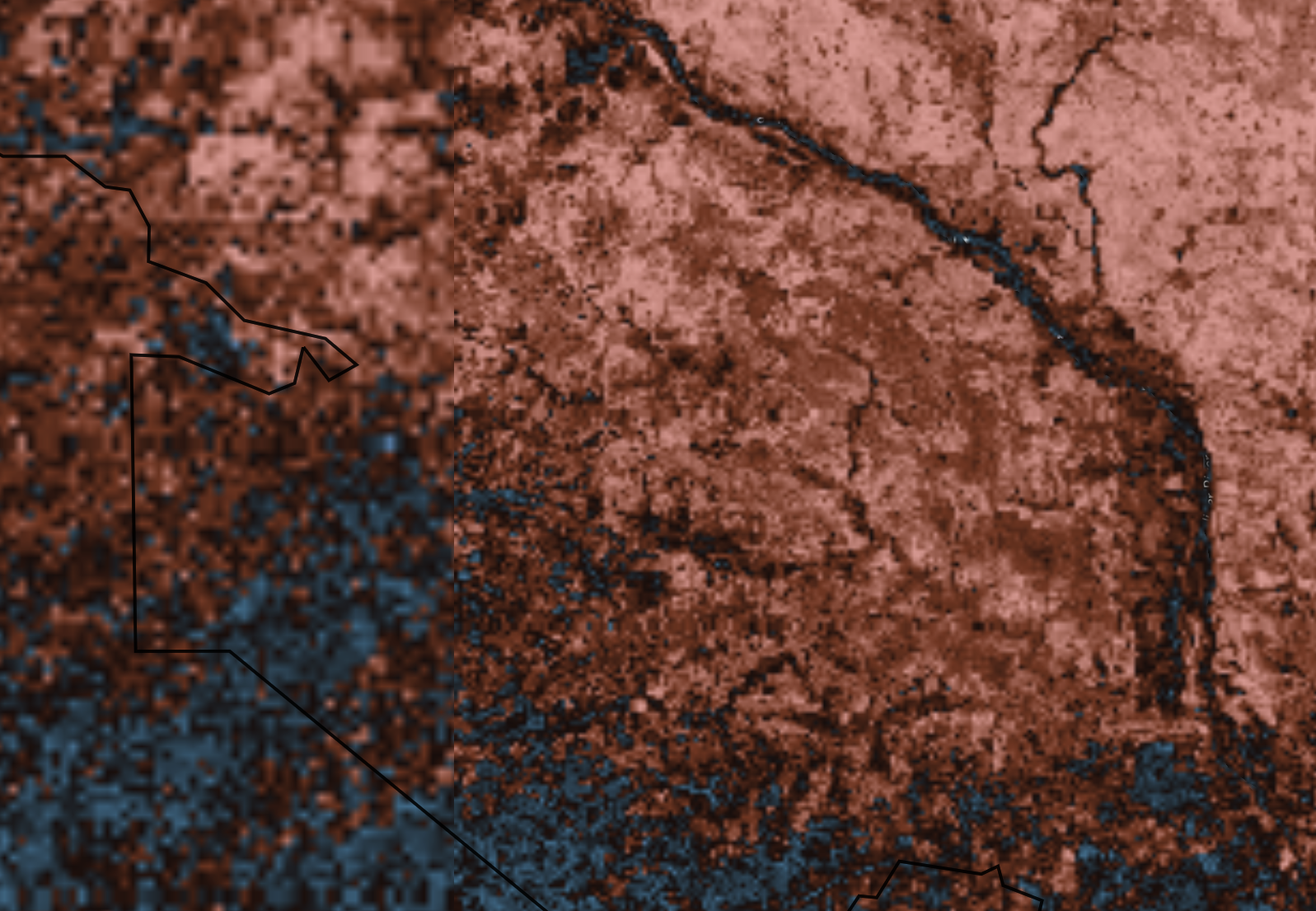
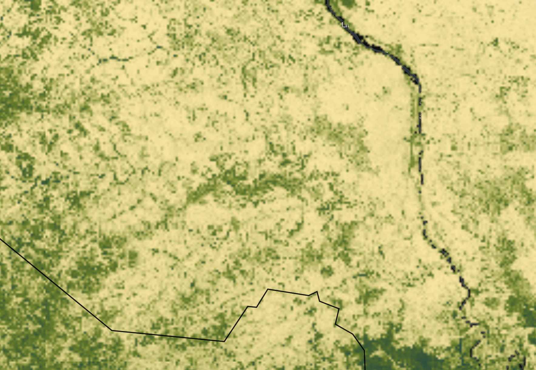
Figure 1. Examples of soil and land health indicators used to support restoration planning.

Spatial analysis allows these indicators to be linked to specific locations. It helps move from a simple data table towards a more geographical understanding of patterns, priorities, and restoration needs.

Getting started

Before you begin, read the steps below carefully.

1. Download the notebook

Click the button below to download the notebook .qmd file.

Download the notebook

2. Open the notebook in RStudio

Open RStudio on your computer.

Then:

Click File → Open File

Select the .qmd file you just downloaded

The notebook will open in RStudio

Make sure you are working in the correct project folder

3. Follow the steps in the notebook

The notebook is structured as a guided workflow. Simply follow the instructions step by step to begin working with land health, soil health, and spatial workflows in RStudio.