2.2 Exploring and evaluating spatial evidence
2.1 explores how spatial evidence is generated and the different degrees of transformation involved including examples of direct measurements, derived indicator/indices, temporal summaries, and modelled predictions. Each of these steps introduces its own inputs, assumptions, and potential for error to enter or compound.
In this section we’ll explore some of the critical considerations (2.2.2), that should be made when working with spatial evidence including data input quality, disclosed uncertainties, spatial and temporal resolution, and more. This prepares us for getting hands-on with data and tools in Module 3.
2.2.1 Working with spatial evidence - critical considerations
Below are a set of practical questions to understand the quality, limitations, and appropriate use of any spatial evidence. While not exhaustive, they provide a good starting point for interrogating a dataset and working with it responsibly.
01 · What?
What is being measured?
Identify the variable or indicator and what it is intended to represent. A vegetation index? Rainfall trend? Soil organic carbon? Consider the unit of measurement being used here - does it make sense?
02 · Where?
What data sit behind it?
What is the input data and where did it come from? Satellite observations? Field sample points? A combination? Is source data disclosed and/or available?
03 · How?
How has it been transformed?
Look for information about the source data, processing methods, models, reference period and validation. Consider how the data has been transformed and whether the methods make sense.
04 · Scale
Where and when does it apply?
Check the spatial resolution, geographic coverage and reference period. Consider whether the scale of the evidence is appropriate for the question or decision at hand.
05 · Confidence
How reliable is the evidence?
Check whether accuracy or validation statistics are reported, and whether an uncertainty layer is available. Model confidence can bias some areas over others.
06 · Fitness for purpose
Is it appropriate for the decision?
Is this piece of evidence actually appropriate for my decision? Could it be corroborated with other kinds of evidence - local knowledge? Other datasets?
In practice we can’t independently verify every one of these for every dataset we use. Research institutes and other authoritative providers do most of this work for you and should publish clear metadata, methods, and validation information and so on, so the answers are there if you go looking. The K4GGWA Evidence Pipeline described in 2.1.2 is designed to support this.
2.2.2 Example maps and interpretation
Below are three example maps - an EVI trend map, a precipitation map, and a soil organic carbon map - each have been produced using different input data, methods and degrees of transformation of raw data to final output.
Work through these three examples with reference to the above, considering what the variable is, what data and methods sit behind it, and in the case of the predictive map example, what the reported accuracy is. Make note where this information is not available, and consider how you might consider this in your decision-making and communication of the evidence.
Enhanced Vegetation Index (EVI)
The Enhanced Vegetation Index (EVI) is calculated using satellite imagery, by measuring how much red and near-infrared light is reflected by the surface of the land, correcting for atmospheric and other distortions. Healthy, dense vegetation reflects this light in a distinctive way, so the index gives a simple measure of vegetation greenness for every pixel in an image. The processing involved is minimal, satellite reflectance values go into a standard formula and a “greenness” value comes out.
EVI maps are therefore close to direct observation but are limited in that they only show greenness across a landscape, not the underlying reason for it. A landscape may appear greener for many different reasons - because of good rainfall or higher CO2 atmospheric concentrations, the spread of an invasive species, or recent changes in land use. When interpreting an EVI map, it is a good idea to look at other evidence alongside, such as rainfall data or land cover information, rather than reading greenness as a direct measure of land health on its own.
Map specifications and metadata
This EVI layer is derived from MODIS (Moderate Resolution Imaging Spectroradiometer), an optical sensor on board NASA’s Terra and Aqua satellites. MODIS observes the entire globe roughly every 1-2 days at a spatial resolution between 250m - 1km, giving it one of the longest continuous vegetation monitoring records available, dating back to 2000. The index shown here is calculated directly from observed surface reflectance, with no field data or modelling involved beyond the standard EVI formula. Since it is a trend map, it summarises the change in EVI over time for each pixel using a simple linear regression, rather than showing a single measurement. Spatial resolution for this map is 500m, and trend period is 2001 - 2024.
Precipitation
A map showing average annual rainfall is typically produced by taking a long record of observed or interpolated rainfall data and calculating the mean at each pixel across that time series. This is one step removed from the raw rainfall data, as it involves summarising many years of values into a single value, and may involve some interpolation or modelling to fill in gaps where there are no direct observations.
The result is useful for understanding the general rainfall pattern across a landscape, including which areas are typically wetter or drier, though it does not show how rainfall is changing over time, only what it has tended to look like on average. Its limitations come from the quality and length of the underlying rainfall record, particularly in regions with few weather stations, where rainfall data is often interpolated or modelled to fill gaps between sparse observations (much of the GGW!). An average that is based on dense weather station coverage in an area may have higher confidence in those numbers than the same average in an area where it relies heavily on interpolation, although not necessarily.
Map specifications and metadata
This map is built from CHIRPS (Climate Hazards Center InfraRed Precipitation with Station data), a daily, 0.05° resolution rainfall dataset that combines satellite infrared observations with ground-based rain gauge records, produced by UC Santa Barbara’s Climate Hazards Center. CHIRPS covers Africa from 1981 to the present. The map shown here represents average annual precipitation, summarised across the full time series at each pixel.
Soil organic carbon (SOC)
Soil organic carbon cannot realistically be measured everywhere across a landscape, so a wall-to-wall SOC map is usually produced through some kind of modelling. Field samples of soil carbon are collected through soil surveys, then linked to other spatial variables that are available everywhere, such as rainfall, topography, and vegetation cover. A model learns the relationship between the field samples and these variables, and applies that relationship across the full landscape to estimate SOC values where no sampling or ground data is available.
The reliability of that prediction depends on how many field samples were used, how well they represent the range of conditions across the landscape, how well the model’s assumptions hold in areas very different from where the samples were collected. This is an example of a kind of variable that can’t be sensed directly from a satellite the way greenness or surface temperature or other variables can.
Map specifications and metadata
This SOC map is produced using machine-learning modeling trained on field soil samples from the Land Degradation Surveillance Framework (LDSF) database, alongside a stack of satellite-derived covariates such as rainfall, topography, and vegetation indices.
Because soil organic carbon cannot be measured with just reflectance values, this kind of model is necessary to extend a limited number of field samples into a continuous, landscape-wide prediction (~85% accuracy). The accuracy of the resulting map depends on the model having been properly trained and validated against independent field data. Spatial resolution is 500m and the reference period is 2023, though the field samples used to train the model were collected over a longer period of time.2.2.3 Communicating uncertainty and limitations
If we understand the accuracy, uncertainty, and limitations of a piece of evidence, we can communicate these alongside our findings and reporting around decisions.
If, for example, a map product has an estimated accuracy of ~ 85%, we may consider combining it with other sources of evidence to corroborate and strengthen the finding. Similarly, if we observe a greening trend in a vegetation condition map we may report that we observe this trend but can’t ascertain the cause and may need ground-truthed data to confirm the species responsible for the greening.
Where available, we should also report relevant information such as validation results, confidence or uncertainty layers, spatial resolution, data coverage, and other known limitations. Where this information isn’t available, we can report this as an uncertainty of itself. This ensures we don’t over-index on any single source of evidence, and that we are transparent about the limitations of the evidence we are using to support our decisions. A more detailed review of spatial evidence quality, limitations and communicating uncertainties can be accessed here.
Stakeholder Approach to Risk-Informed and Evidence-Based Decision-Making (SHARED) Toolkit

The SHARED Toolkit can be consulted as a comprehensive guide on achieving inclusive, evidence-based decision-making in restoration work. In particular Phase 2 - Integrating Evidence and Experience can be consulted for further guidance on the process of engaging diverse stakeholder groups, integrating multiple sources of evidence, and communicating uncertainty and limitations in a transparent and effective way.
This resource goes beyond the scope of this tutorial, but is a useful reference for those interested in the broader context of evidence-based decision-making in restoration.
2.2.4 Ready to work with the data?
We’ve now explored the different types of spatial evidence, formats, how they are generated, and how to evaluate quality and limitations.
Next, we move from understanding and evaluating spatial evidence to actually working with it! In Module 3, we’ll explore our spatial data ecosystem including where to discover GGW datasets, how our open-data infrastructure provides access to them, and how you can begin working with them using R and other tools.
Knowledge check
Q1. Which of the following is a modelled or predicted variable, rather than a direct measurement or a simple index?
Q2. Why is it useful to check the provenance of spatial evidence?
Q3. What does responsible communication of uncertainty look like?
Learn more
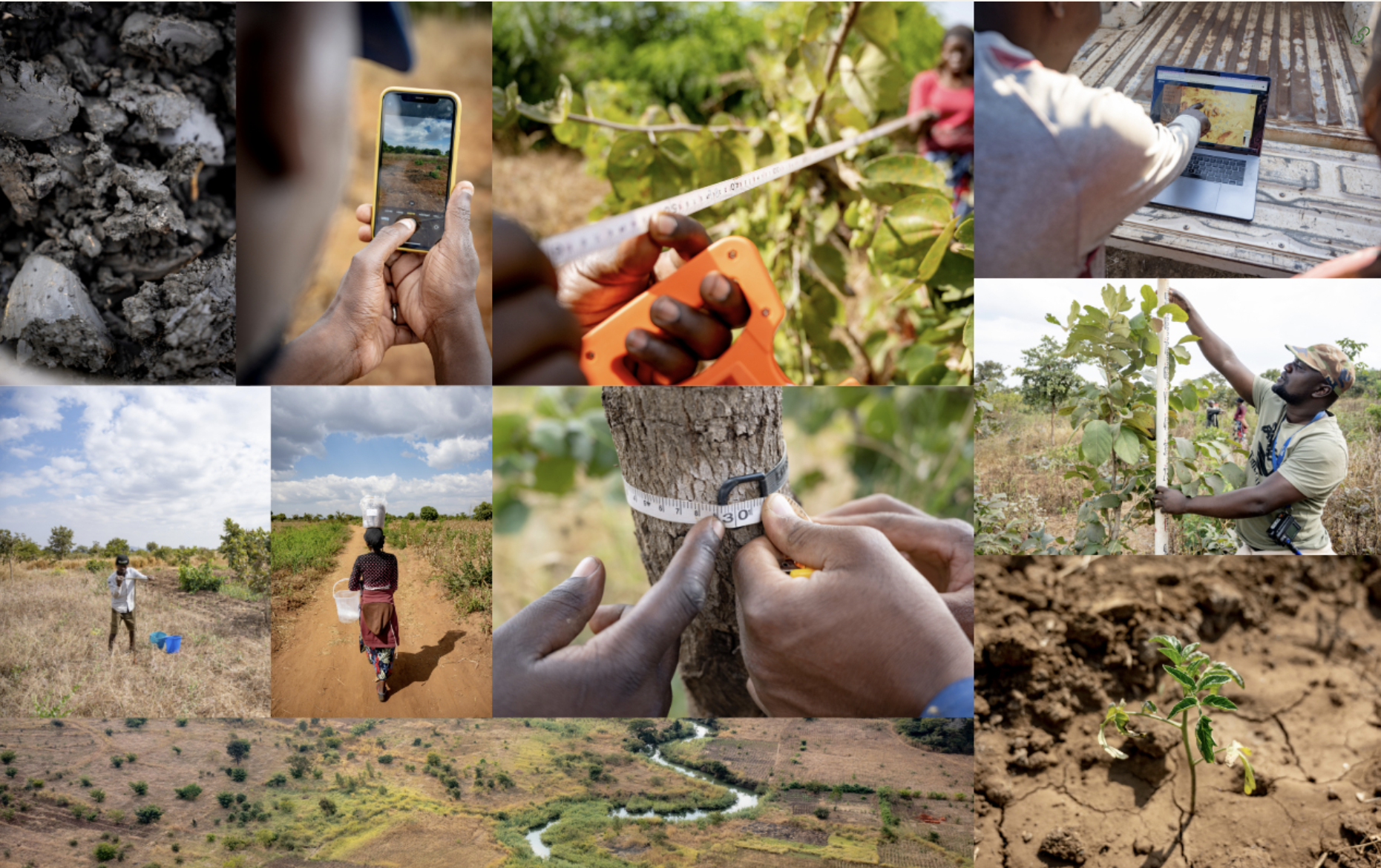
Land Degradation Surveillance Framework
Spatial data
Learn about the Land Degradation Surveillance Framework (LDSF), the world's most widely deployed systematic, standardised approach to collecting and analysing spatial data for restoration monitoring and reporting.
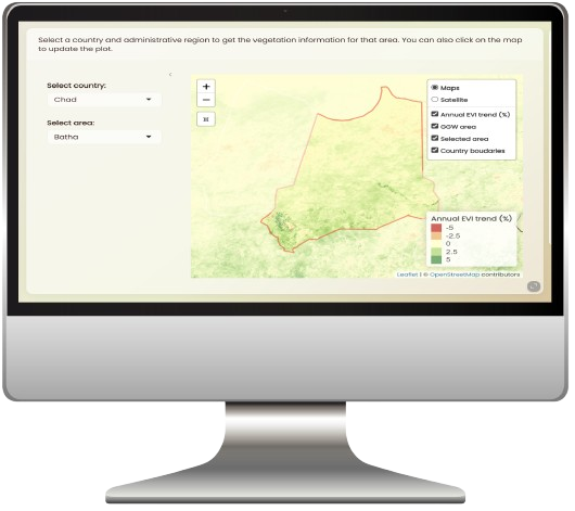
GGW dashboards
Dashboard
Explore land health dashboards for the Great Green Wall, which provide visual summaries of spatial evidence on land health and restoration progress across the region.