2.1 How spatial evidence is generated
In 1.3, we looked at how spatial evidence is produced and how different data sources, methods, and assumptions can all affect what a map is showing and how confidently it can be used.
This section builds on that foundation in three parts: a general workflow of raw data or observations to evidence, different formats of spatial evidence, Earth observation as an increasingly important source behind many spatial evidence products, and, finally, the specific steps used to generate the datasets behind this hub, from field to open data.
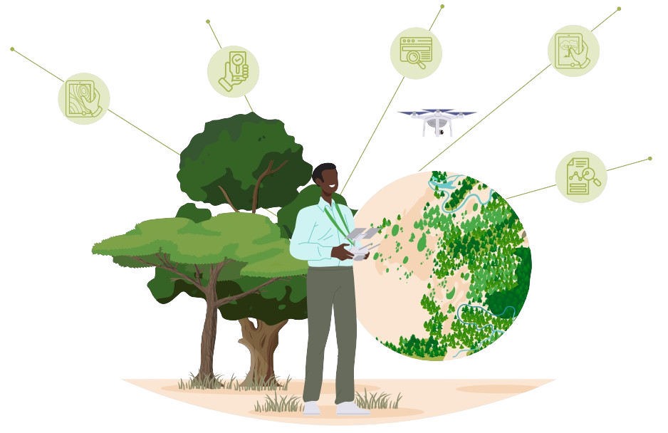
2.1.1 From observations to evidence
In the context of landscape restoration, spatial evidence is the analysed or modelled output derived from spatial data (data with locational information) that helps describe landscape conditions and trends, and inform decisions. It may be presented in a range of formats including as static or interactive maps, charts, plots, in dashboards, summary tables, and other visualisations. This hub focuses mainly on spatial evidence presented as maps, though the same principles apply to interpreting any of these formats.
Spatial evidence is ultimately a product of different kinds of observations of the world coming from a wide variety of sources - satellites, aircraft, weather stations, direct field samples, IoT sensors, household surveys, citizen-science data, and more.
Getting from a raw observation to a usable piece of evidence almost always involves some degree of processing, transformation, or combination with other data. In our data-rich world, spatial evidence products increasingly combine several sources to produce richer, more informative outputs.
Observe Collect data/observations of the world
satellites · field data · sensors
Process Prepare and quality-control data
correction · cleaning · calibration
Analyse / model Transform, combine, analyse data
indices · summaries · comparisons · predictions
Product Represent the information across space
maps · indicators · datasets
Evidence Interpret in relation to a question or decision
Spatial evidence as raster (and other) data
Spatial evidence is usually represented in one of two main formats: raster or vector.
A raster represents a landscape as a continuous and regular grid of cells (pixels), with each cell storing a value. This makes raster data the best format for capturing continuous and sometimes categorical variables.
A vector represents discrete features using either points, lines and polygons. Points might represent field observations or sampling sites; lines could represent rivers or roads; and polygons might represent fields, protected areas, administrative boundaries or restoration project areas.
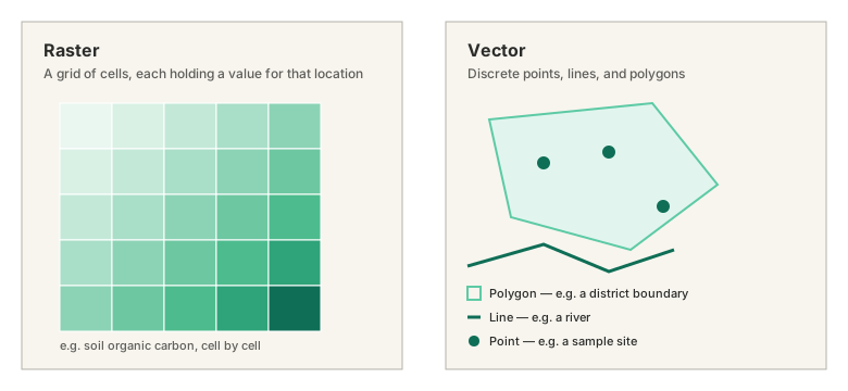
Why do we work so much with raster data?
Environmental conditions are typically continuous variables - meaning their observable properties tend to change and vary continuously across whole landscapes. A raster allows us to represent this continuity by storing a value for every pixel across the landscape.
This is also how much of our spatial evidence is generated - Earth observation satellites measure the Earth’s surface as grids of pixels and, often as a function of that, statistical and machine-learning models used to estimate environmental conditions across areas often produce their results in the same gridded format. Raster data is particularly useful for comparing conditions across large areas, identifying spatial patterns and trends, and combining multiple environmental indicators.
Raster and vector data are often used together. For example, we might use a raster map to visualise vegetation condition across a whole country and overlay vector boundaries to summarise values within districts, restoration sites or other areas of interest. Read more about spatial data data formats here.
Earth observation: a growing, increasingly essential input
Earth observation (EO) - repeated satellite and aerial imagery of the Earth’s surface - is one of the most important data sources feeding into spatial evidence.
Historically, it was expensive and controlled by a small number of national space agencies but over the past couple of decades this has changed substantially with a rapidly growing number of public and commercial satellite missions, combined with free and open data policies from major providers, meaning that consistent, repeated observations of the Earth’s surface are now openly available, at increasing spatial and temporal resolution, across almost the entire globe.
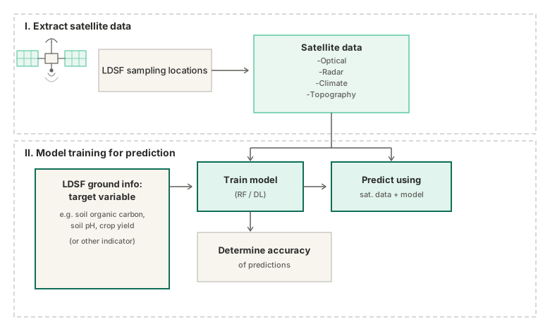
EO data on it’s own can sense and measure physical properties of the Earth’s surface like reflected light, radar backscatter, but is incapable of measuring things like soil organic carbon, woody biomass, or biodiversity, all of which typically require ground-sampling to train and validate models. The combination of EO and field data is very powerful, enabling us to produce spatial evidence that is both spatially continuous and grounded in real-world measurements.
Different degrees of transformation
From direct measurements to derived indicators, temporal summaries, and modelled predictions, progressively more processing steps are involved and, with each step, more assumptions are introduced and more opportunity exists for error to propagate and compound. 2.2 picks this up in more detail, working through concrete examples and technical considerations to make when using spatial evidence to support decisions.
2.1.2 The K4GGWA evidence pipeline
The general process described above applies directly to how the evidence products available on the K4GGWA platform are generated. Below we step through that pipeline, from systematic field sampling through laboratory analysis and modelling, to open data access and decision-making.
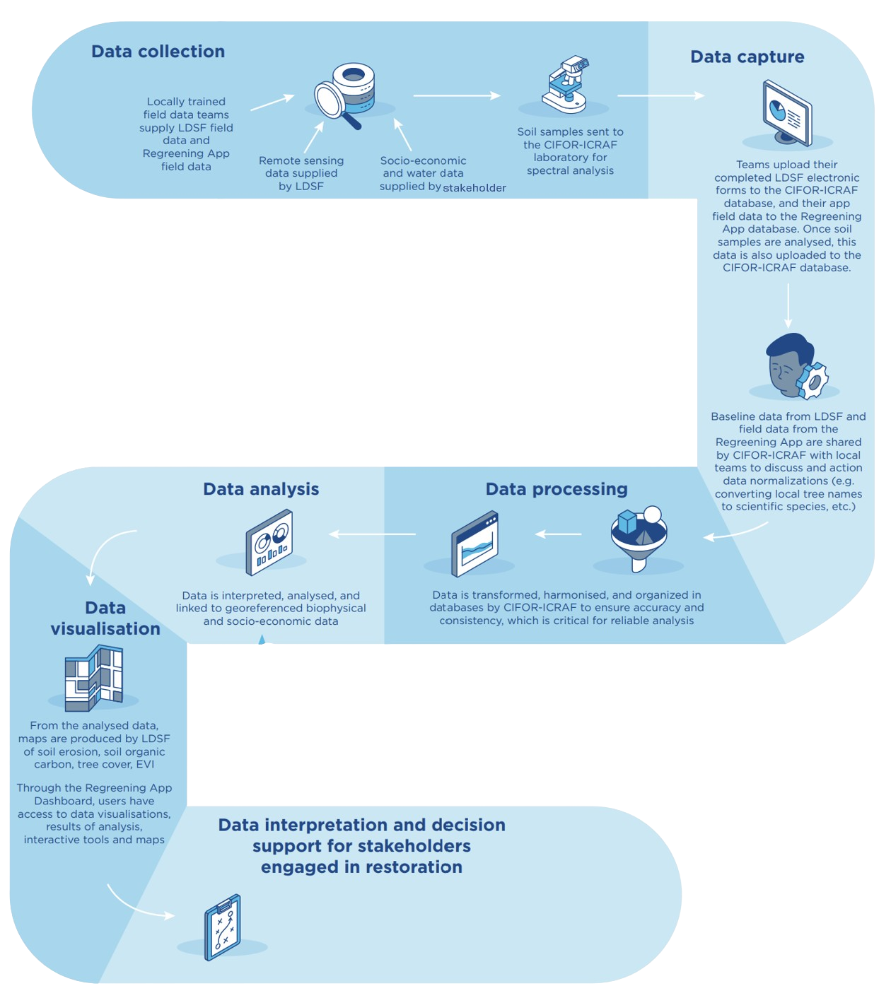
For a more detailed step-through of the process followed to generate the soil and land health evidence products available on this hub, explore the steps below, as well as the Papers and Methods section for more technical details on the methods used to generate the datasets.
K4GGWA Soil and Land Health Monitoring Pipeline
LDSF - Systematic field sampling
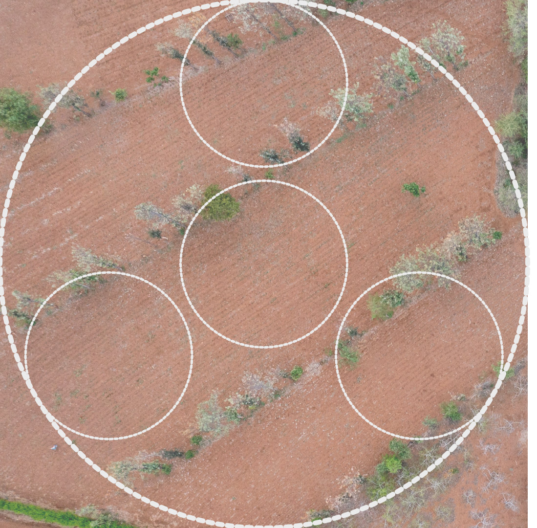
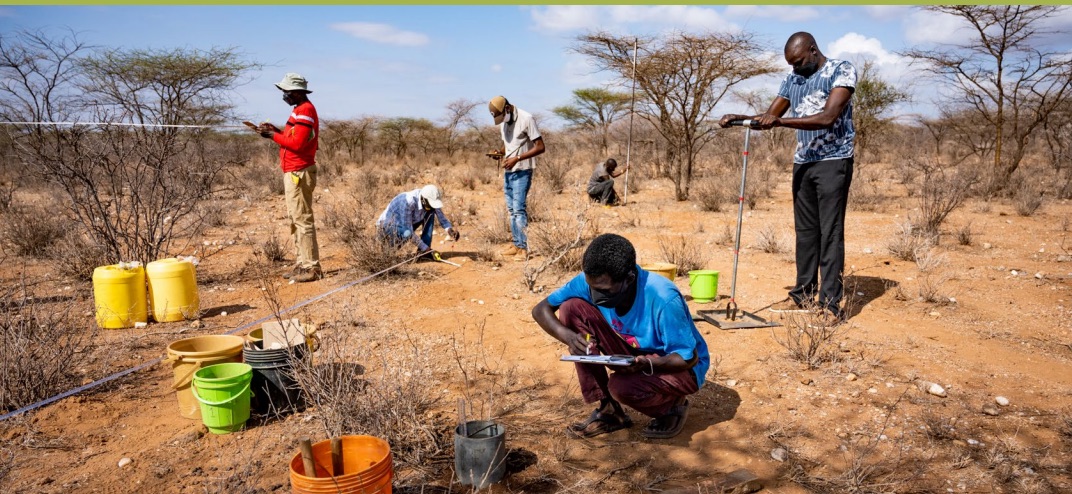
Field data collection follows the Land Degradation Surveillance Framework (LDSF) - a systematic, nested sampling design used across Africa's diverse landscapes, including throughout the GGW countries.
Sites are selected at random within a landscape. Each site is a 10km x 10km quadrat containing 16 clusters, each made up of 10 plots, each in turn divided into 4 subplots. This nested, multiscalar design captures spatial variation at several scales within the same landscape, which keeps the resulting data minimally biased and makes it a robust foundation for the modelling described later in this pipeline.
The framework is designed to collect soil and land health data like erosion prevalence, soil physico-chemical properties, and biodiversity, but may be extended with additional modules depending on the context, for example, using the rangeland or eDNA modules, so the same underlying design can be adapted to different landscape and monitoring needs.
Regional soil analysis labs
Alongside physical soil samples, field teams record observational data directly through a digital (ODK) form including erosion prevalence and other visually assessed indicators, identified plant species, biomass measurements, and more. This means every physical sample is paired with rich, geolocated field observations.
Physical samples are transported either to the main laboratory facility at World Agroforestry in Nairobi, or to one of a growing network of regional soil labs part of ongoing efforts towards regional lab capacity building.
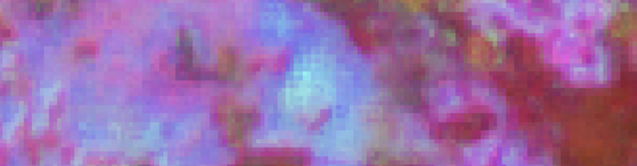
In the lab, samples are processed through our Lab Information Systems (LIMS), and analysed using state-of-the-art spectroscopy alongside other equipment, enabling high-throughput, high-accuracy analysis at a scale that would not be feasible using conventional wet-chemistry methods.

Building the LDSF database
Laboratory results and field-collected (ODK) observations are processed, cleaned, and quality-controlled, then integrated into the LDSF database.
This database, which comprises Africa's largest soil spectral library, alongside associated plant and land health data, are the reservoir that all downstream analytical products are drawn from. Everything described in the next two steps depends on the quality and consistency established at this stage.

Analyses and predictive modelling
The LDSF database is used to train deep learning models of land health combining field-referenced measurements with Earth observation imagery and other environmental covariates (see the note on Earth observation above) to predict conditions continuously across the landscape, not just at sampled locations.
This is the same points-to-predictions step introduced in the general workflow above, applied at scale, using advanced models to generate continuous raster products together with explicit measures of uncertainty, for visibility over predicted value at any location and confidence in the output.
Open data access
The resulting data products are published through an open, STAC-based data infrastructure, including a dedicated GGW catalog that is interoperable, transparent, and FAIR, such that maps, metadata, and underlying assets can be reused across different workflows and decision contexts.
For many GGW-relevant indicators, these products outperform available global default datasets, and technically capable practitioners can go further still by combining and building on the underlying data to generate their own evidence.

In the next section 2.2 we explore practical questions and considerations when integrating evidence into our decisions - covering the quality and possible biases of the underlying data, transformation steps involved in producing the final output, metadata availabilities to verify any of this, and practical questions about the evidence itself including what variable is represented, the unit of measurement, the spatial and temporal resolution, and how it might be combined with other evidence to support a more informed decision.
Learn more
Learn about the Land Degradation Surveillance Framework (LDSF) and the pipeline used to generate the soil and land health evidence products available on this hub.
Explore and learn more about different kinds of geospatial statistical modeling methods and transformations, including regression, interpolation, and machine learning.